Sea level has never been constant throughout Earth’s history. It has risen and fallen over geological time due to various natural processes. This blog explores the cyclic patterns of sea level fluctuations in the geologic past, the role of oxygen isotopes, and the contribution of marine organisms in reconstructing ancient sea levels.
Cyclic nature of sea level in geologic time:
The sea level is always in a dynamic state and was not static in the geological past. Analysis of sedimentary data, ancient benchmarks, raised beach, and wave cut notches in stable areas of geologic cliff sections indicates that sea level changed periodically in a cyclic order. Several sea level curves are available in the published literature.
There are many quests to draw more accurate sea level curves that are worldwide acceptable. Figure 1 shows that the amplitudes of sea level rise in the early geologic time (Paleozoic) were much higher than the present (Quaternary).
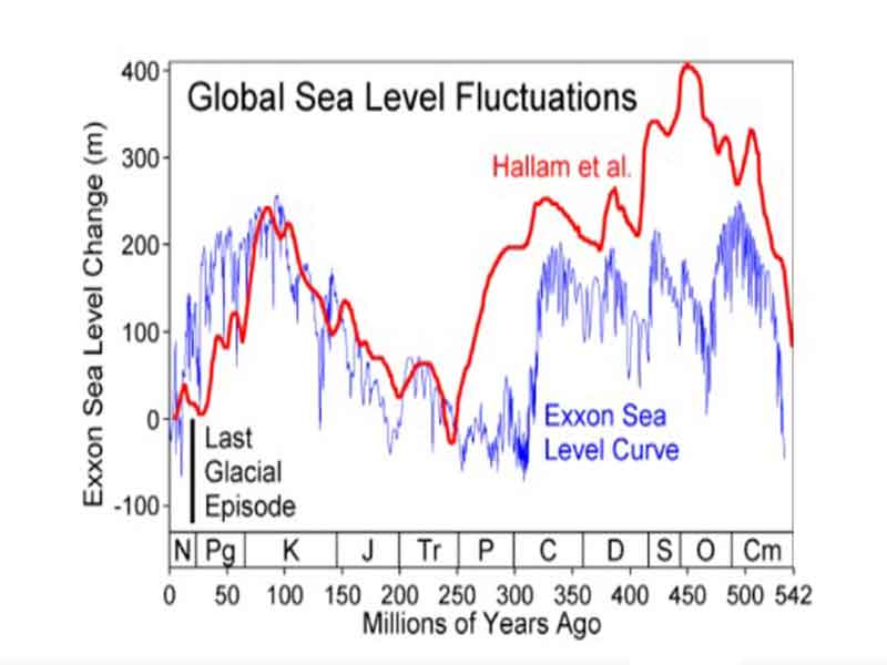
Fig. 1: Variation of the sea level during the Phanerozoic eon. (Source: Wikipedia. This figure was prepared by Robert A. Rohde from publicly available data and is incorporated into the Global Warming Art)
Oxygen isotopes and sea level estimation:
The fractionation of oxygen isotopes and the process of formation of foraminifera shells play a vital role in estimating the paleo-Sea Surface Temperatures (SST), as well as the sea level fluctuations. The oceanic water contains both 16O and 18O.
During evaporation lighter 16O evaporates faster than heavier 18O and in the glacial period in high latitudes, evaporated vapor from the ocean contains higher percentage of 116O compare to 18O. Therefore, the concentration of 18O in oceanic water increases and hence, the remaining water becomes concentrated.
So, there is a connection between temperature and sea level. The 18O/16O ratio provides a record of ancient water temperature. During the glacial period, oceanic water evaporates and evaporated vapor after cooling accumulates on the land surface in the form of an ice sheet when the sea level drops (lower).
During the cold period, cold water containing higher content of 18O spreads toward the equator and hence, water vapor rich in 18O preferentially rains out at lower latitudes in comparison with the high latitudes.
The remaining water vapor that condenses over higher latitudes is subsequently rich in 16O. Therefore, glacial ice contains water with a low 18O content. Since large amounts of 16O water are being stored as glacial ice, the 18O content of oceanic water is high.
Alternatively, water up to 5°C (9°F) warmer than today represents an interglacial, when the 18O content of oceanic water is low. Therefore, 16O in oceanic water becomes high. This principle has been adopted in drawing sea level curves.
Foraminifera: The Oceanic Thermometers:
Variation of the sea level during the Phanerozoic eon. (Source: Wikipedia. This figure was prepared by Robert A. Rohde from publicly available data and is incorporated into the Global Warming Art.
One of the best records of paleo-ocean temperatures can be found in the shells of marine creatures called foraminifera. Foraminifera are called oceanic thermometer. Their shells are used to measure paleotemperature. Planktonic foraminifera are very tiny sea organisms that produce calcium carbonate (CaCO3) shells to protect themselves.
When they make their shells, they incorporate oxygen from the oceanic water, which contains both 16O and 18O. The ratios of delta 16O and 18O change due to the changes in sea surface temperature. After death, their shells fall on the ocean floor along with the oceanic sediments.
Based on 18O value obtained from foraminifera shells found in oceanic sedimentary sequences, scientists have been able to reconstruct historic sea surface temperatures (SSTs) at the time of the shells’ formation.
Shackleton and Opdyke’s isotope curve:
The Oxygen isotope curve of Shackleton and Opdyke (1973) has been constructed based on the 18O values obtained from Core Vema 28-238 (Fig.2). This is an excellent oxygen isotope and magneto-stratigraphy curve.
The curve has been drawn collecting undisturbed oceanic sediments deposited continuously through the past 870,000 years. A detailed correlation with sequences described by Emiliani (1961, 1966) in the Caribbean and Atlantic Ocean is demonstrated.
The boundaries of 22 stages representing alternating times of high and low Northern Hemisphere ice volume are recognized and dated. The record is interpreted in terms of Northern Hemisphere ice accumulation and is used to estimate the range of temperature variation in the Caribbean.
This curve has been regarded as the Pleistocene sea level curve. Oxygen isotope curve (Opdyke and Shackleton, 1973) has 22 stages. Odd numbers represent Interglacial or warm phases and even numbers represent Glacial or cold phases. Warm phase indicates high sea level and cold phase indicates low sea level. Hence, the curve represents the curve of the sea level changes for 1.5 ma.
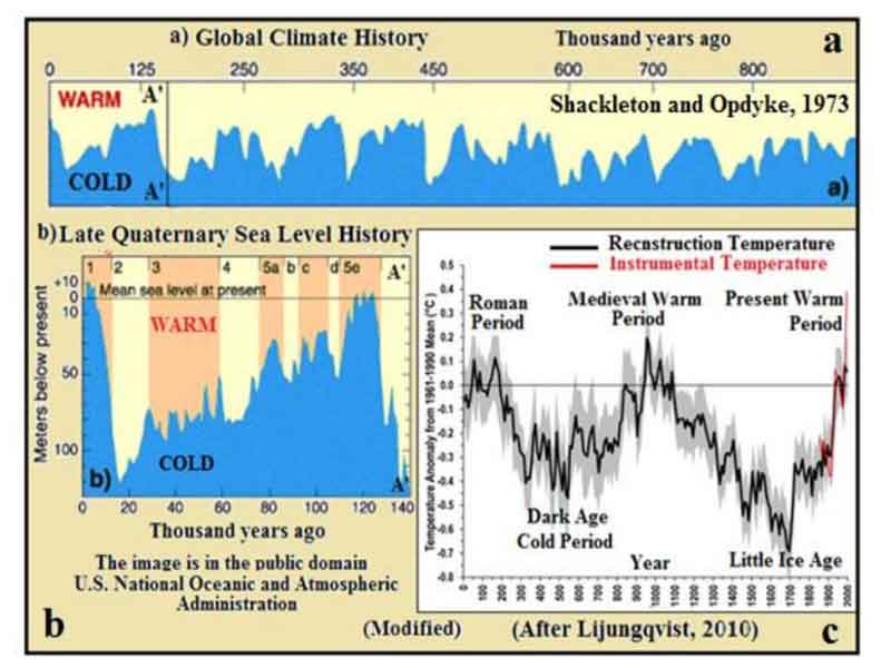
Fig.2: Oxygen isotope curve of Shackleton and Opdyke (1973). The curve has been regarded as the Pleistocene sea level curve.
Sea level during the last glacial maximum:
During the Last Glacial Maximum (about 18,000 years BP), the sea level was about 100m to 140m below the present sea level. English Channel (separates the British Isles from the mainland) and Bering Strait (which separates the Eurasian and American continents) were dry.
It was the time when most probably, our ancestors migrated from Asia to America. After the Glacial Maximum, global climate started to warm up and thick ice sheets on continental interior started to melt down.
Melting water discharged into the ocean basins through deeply incised river valleys and consequently, sea level started to rise. In fact, there are two schools of thoughts in context of Holocene sea level curves. A group of scientists are in favor of plotting smoothly rising sea level curves, whereas the other group supports the rapidly rising sea level.
Holocene sea level curve and proxy data:
The Fig. 3 shows the sea level curve starting from the Late Pleistocene to Holocene. The sea level curve was drawn by compiling dataset from different regions and from several sets of proxy data. The data gather from natural recorders of climate variability, such as, ice core, fossil pollen, tree rings, varve, corals and historical or archeological materials etc. are called proxy data.
The curve shows a smooth upward rise of sea level from the Last Glacial Maximum up to 15,000 years BP, and thereafter a sharp sea level rise reached its present position at about 8000 years BP.
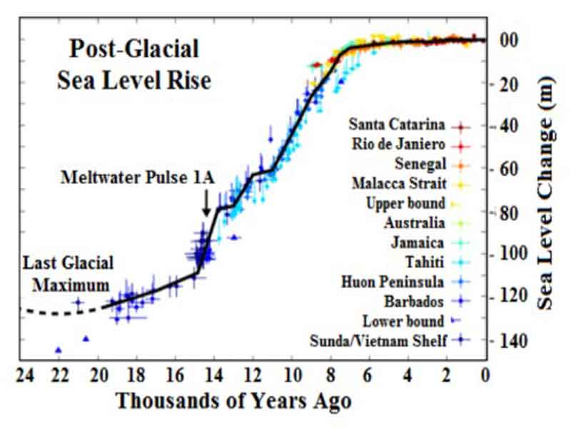
Fig. 3: Rise of sea level after Last Glacial Maximum (LGM). Source: Image created by Robert A. Rohde. The original work was created for the Global Warming Art Project (Wikipedia).
Conclusion:
Reconstructing past sea level changes helps us understand Earth’s climatic evolution and predict future scenarios. From foraminifera shells to isotope ratios, the geological record holds the keys to interpreting sea level fluctuations—valuable insights that bridge the ancient past to the changing climate of today.